
Mapping Network Access
Using OpnSense and Grafana

Your router connects your devices to the world—but do you really know where your network traffic is going? Every device on your network, whether it's your laptop, TV, or smart lighting, is constantly sending and receiving data. Some of these connections are expected, like accessing cloud services or streaming media, but others might raise red flags. What if your laptop is silently exfiltrating your sensitive data to a foreign server? Or an IoT device is part of a botnet attack against a major corporation? By collecting and analyzing the logs from your network router, you can visualize your network’s footprint in real-time, identify suspicious connections, and gain valuable insights into how your devices interact with the internet.
In this guide, we’ll walk through how to collect and process network traffic data from an OpnSense router using Grafana Alloy and Loki, to display an interactive map on a Grafana dashboard. Whether you’re a tech enthusiast looking to safeguard your home, or a cybersecurity professional, this setup will help you uncover the hidden patterns in your network traffic—before they become a problem.
For this setup, we’ll use the following free and open source tools:
A firewall and routing platform that includes most of the features available in expensive commercial firewalls.
A platform for running applications in a loosely isolated environments called containers. Containers are lightweight and contain everything needed to run the application without needing to rely on what's installed on the host
An OpenTelemetry collector with support for metrics, logs, traces, and profiles compatible with the most popular open source ecosystems
A log aggregation system designed to store and query logs from all your applications and infrastructure
A data visualization and monitoring solution
Installing a router/firewall into your existing network and configuring it to route traffic is beyond the scope of this guide, so we'll assume that you have a working OpnSense or pfSense firewall already in place. If you need to set this up yourself, I suggest following the guides at https://opnsense.org/users/get-started/
The Grafana set of tools will be ran as Docker containers, so if you don't have Docker installed already on your system, head over to https://docs.docker.com/get-started/get-docker/ to find the installation that best suits your system.
With Docker installed, each of the Grafana tools can be installed with a single Docker Compose file.
version: "3.3"

services:
  alloy:
    container_name: alloy
    image: grafana/alloy:latest
    ports:
      - 12345:12345
      - 1514:1514
    command: run /etc/alloy/config.alloy --server.http.listen-addr=0.0.0.0:12345 --storage.path=/var/lib/alloy/data
    volumes:
     - alloy_data:/etc/alloy

  loki:
    container_name: loki
    image: grafana/loki:latest
    ports:
      - 3100:3100
    command: -config.file=/etc/loki/local-config.yaml

  grafana:
    container_name: grafana
    image: grafana/grafana:latest
    ports:
      - 3000:3000
    volumes:
      - grafana_data:/var/lib/grafana

volumes:
  alloy_config:
grafana_config:First, we need to configure OpnSense to log network traffic. The firewall can log connection events, which will later be collected by Grafana Alloy.
Log into your OpnSense dashboard and navigate to System > Settings > Logging.
Go to the Remote tab and click the + to add a new remote destination.

Click on the Remote tab, and create a new destination with the options below. Port 1514 matches the port exposed in the Alloy section of the Docker Compose file earlier.

Click Save, then hit 'Apply' on the Remote tab to start sending logs to Grafana Alloy.
Before Grafana Alloy can collect the logs from OpnSense, the config.alloy file needs to be configured to receive logs, process them, and write them to Loki. Alloy works using a series of code blocks to configure different components by applying processing stages, before sending the results to the list of receivers. A stage is a tool that can parse, transform, or filter log entries. These stages are applied to each log entry in the order added to configuration file. Documentation for each of the stage blocks used can be referenced at:
The overall config file needs 3 main blocks: a listener to receive log files, a processor to modify the logs, and a write stage to send the modified logs out.
.
Create a new config.alloy file and add a listener block for the OpnSense syslog messages using port 1514. This port was exposed earlier while installing Alloy through Docker.
loki.source.syslog "listener" {
	listener {
		address = "0.0.0.0:1514"
	}
	forward_to = [loki.process.opnsense.receiver]
}
Now we need a processing block that matches the forward_to line of the listener. All of the various processesing stages will take place in this overall processing block.
loki.process "opnsense" {

}
The first processing stage is a regex block that breaks each log line into separate parts. It takes a single parameter, expression, that describes the RE2 regular expression string to be applied to the log line. Each (?P<name>re) section represents a named capture group, with the name used as the key for the matched value. Because of how Alloy syntax strings work, any backslashes must be escaped with a double backslash.
IPv4 and IPv6 has different formats, as do the TCP, UDP, and ICMP protocols in each IP version. A full description of each type of log line can be found at:
stage.regex {
	expression = "^(?s)(?P<fw_rule>\\w*),(?P<fw_subrule>\\w*),(?P<fw_anchor>\\w*),(?P<fw_label>\\w*),(?P<fw_interface>\\w*),(?P<fw_reason>\\w*),(?P<fw_action>\\w*),(?P<fw_dir>\\w*),(?P<fw_ipversion>\\w*),(?P<fw_tos>\\w*),(?P<fw_ecn>\\w*),(?P<fw_ttl>\\w*),(?P<fw_id>\\w*),(?P<fw_pckt_flags>\\w*),(?P<fw_pckt_flags>\\w*),(?P<fw_protonum>\\w*),(?P<fw_protoname>\\w*),(?P<fw_length>\\w*),(?P<fw_src>\\d+.\\d+.\\d+.\\d+),(?P<fw_dst>\\d+.\\d+.\\d+.\\d+),(?P<fw_srcport>\\w*),(?P<fw_dstport>\\w*),(?P<fw_datalen>\\w*),(?P<fw_flags>\\w*),(?P<fw_seq>\\w*),(?P<fw_ack>\\w*),(?P<fw_window>\\w*),(?P<fw_urg>\\w*),(?P<options>.*)$"
}
The next two stages assign labels that we can filter on in our dashboard. Loki is limited 15 labels, so we can't choose everything, and we need to leave some available for the location data. Additionally, labels should only be used for items that have a limited number of options, else performance can be degraded rapidly. That means things like Action (pass/block), direction (in/out), and IP Version (4/6) make good labels, while IP addresses and port numbers are best as structured metadata, attached to a log without being indexed or included in the log line content itself.
stage.labels {
	values = {
		action = "fw_action",
		dir = "fw_dir",
		interface = "fw_interface",
		ipversion = "fw_ipversion",
		protocol = "fw_protoname",
	}
}

stage.structured_metadata{
	values = {
		src_ip = "fw_src",
        src_port = "fw_srcport",
		dst_ip = "fw_dst",
		dst_port = "fw_dstport",
	}
}
To get a location from the IP addresses, we'll utilize the MaxMind databases. Sign up for an account at https://www.maxmind.com and download both of the databases listed here. Be sure to select the GZIP version, as they contain the mmdb files that the item can use.
Extract the mmdd files from each GZIP and copy them to the same location as your config.alloy file. Then setup the initial geoip stage, followed by stages for labels and structured metadata.
stage.geoip {
	db             = "/etc/alloy/GeoLite2-City.mmdb"
	db_type        = "city"
	source         = "fw_src"
}

stage.labels {
	values = {
		src_location = join(
			[
            	"geoip_city_name",
				"geoip_subdivision_name",
				"geoip_country_name",
				"geoip_continent_name",
			],
			", ",
		),
		src_country  = "geoip_country_name",
	}
}
stage.structured_metadata {
	values = {
		src_zipcode = "geoip_postal_code",
		src_latitude = "geoip_location_latitude",
		src_longitude = "geoip_location_longitude",
	}
}
While location is good, from a network analysis perspective, it's also beneficial to know about the server that owns the target IP. A Windows computer reaching out to a Microsoft server? Probably okay. A smart refrigerator reaching out to a VPN provider in China? Probably not.
So, we'll do a second geoip stage using the ASN database, and capture the organization for the IP.
stage.geoip {
	db             = "/etc/alloy/GeoLite2-ASN.mmdb"
	db_type        = "asn"
	source         = "fw_src"
}

stage.labels {
    values = {
    	src_organization = "geoip_autonomous_system_organization",
    }
}
With all of the data collected for the source IP, we'll repeat it for the destination IP.
Note: It should be possible to use match stages to only look get source information for inbound IP connections and destination information for outbound IP connections, but I've been unable to get that to work consistently. Instead, we'll waste the extra cpu time searching for both sets of information even though only one set will return.
stage.geoip {
	db             = "/etc/alloy/GeoLite2-City.mmdb"
	db_type        = "city"
	source         = "fw_dst"
}

stage.labels {
	values = {
		dst_location = join(
			[
            	"geoip_city_name",
				"geoip_subdivision_name",
				"geoip_country_name",
				"geoip_continent_name",
			],
			", ",
		),
		dst_country  = "geoip_country_name",
	}
}

stage.structured_metadata {
	values = {
		dst_zipcode = "geoip_postal_code",
		dst_latitude = "geoip_location_latitude",
		dst_longitude = "geoip_location_longitude",
	}
}

stage.geoip {
	db             = "/etc/alloy/GeoLite2-ASN.mmdb"
	db_type        = "asn"
	source         = "fw_dst"
}

stage.labels {
	values = {
    	dst_organization = "geoip_autonomous_system_organization",
   	}
}
Lastly, add a line pointing to the writer block that will send all of our data to Loki.
forward_to = [loki.write.default.receiver]
With the processing done, the logs need to be sent somewhere. For this, we direct them to our Loki install as shown below. Just make sure to change the IP address to match that your Docker host.
loki.write "default" {
	endpoint {
		url = "http://<dockerhost_ip_address>:3100/loki/api/v1/push"
	}
}Once Alloy is receiving logs, we need to store them using Loki. Loki, like Alloy, uses a configuration file to compose its settings. These first few settings below control the overall server as a whole. Copy them into a new yaml file.
auth_enabled: false

server:
  http_listen_port: 3100
  grpc_listen_port: 9096
  log_level: debug
  grpc_server_max_concurrent_streams: 1000

common:
  instance_addr: 127.0.0.1
  path_prefix: /tmp/loki
  storage:
    filesystem:
      chunks_directory: /tmp/loki/chunks
      rules_directory: /tmp/loki/rules
  replication_factor: 1
  ring:
    kvstore:
      store: inmemory
The next group of settings are more general purpose configurations. Since we're using structured metadata in our Alloy configuration, make sure that allow_structured_metadata is set to true.
query_range:
  results_cache:
    cache:
      embedded_cache:
        enabled: true
        max_size_mb: 100

limits_config:
  metric_aggregation_enabled: true
  allow_structured_metadata: true

ruler:
  alertmanager_url: http://localhost:9093

frontend:
  encoding: protobuf

analytics:
   reporting_enabled: false
Lastly, add a set of configurations to manage our specific schema. All logs after the from date will use these settings. Additionally, structured metadata was included in v13, so if you're modifying an existing configuration, make sure to change the schema version. Finally, ensure that the port listed in the loki_address matches the http_listen_port earlier, and the endpoint used in the Alloy configuration.
schema_config:
  configs:
    - from: 2020-10-24
      store: tsdb
      object_store: filesystem
      schema: v13
      index:
        prefix: index_
        period: 24h

pattern_ingester:
  enabled: true
  metric_aggregation:
loki_address: localhost:3100Now that all of the heavy work is done, we can do the fun part of creating a map to display the geographic locations of each IP connection.
In Grafana, open up the Menu and click on the Add New Datasource button near the bottom. In the list of available sources, search for Loki. You can give the source a name, or keep it the default. Add the URL to your Loki instance, and then scroll all the way to the bottom and click the Save & Test

Click on the Build a dashboard button, and we can finally start visualizing our data. For me, I want to know two things:
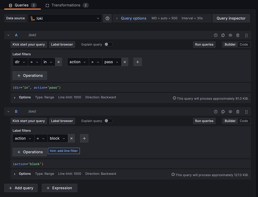
This means I need to come up with two queries. Once Loki is selected as the data source, the dropdown in the label filters will populate with the labels we created in our Alloy config file. Creating a query that filters on two labels, direction = in and action = pass, will only show inbound connections. Creating a second query that filters action = pass, will show blocked connections, regardless of direction.
In the top right corner of the screen is the option for which type of visualization is shown. It defaults to Time but, near the bottom of the list, is an option for a Geomap, which will automatically place markers onto a map for any latitude and longitude field it finds. Since we have two sets of latitudes and longitudes, we have to help the software out a little by transforming our data.
We need two transformations added to our data. The first is to extract the structured metadata from our log. Add an Extract Fields transform, set the source to Labels and toggle the option to replace all fields. Now all of the data in our log will be visible for our use, not just the regular labels. However, each of these fields are formatted as strings. The Geomap expects latitude and longitude fields to be numbers. Add a Convert Field Type transform, select each latitude and longitude field, and set them each as Number.
Now, we can set the Geomap to use these fields as our latitude and longitude source. In the Geomap configuration panel on the right, Configure the markers layer to use coordinates, then set the latitude and longitude fields appropriately.

Since each marker is partially opaque, locations that have more connections in the log appear more solid. However, it's even easier to see which locations are more active by changing the layer type to Heatmap. Just reselect the latitude and longitude fields, and leave the other settings alone, and you can get a result like below.

These maps are only displaying the data from Query A. By adding a second layer, the data from the second query can be displayed. In the map below, both blocked and allowed IP addresses are shown, with a separate color for each group.

Whether you’re monitoring security threats or just curious about where your network traffic is going, mapping the IP addresses found in your router's logs instantly transforms meaningless numerical data into geographical information that provides powerful insights into your network activity and helps to shape the decisions on how best to secure it, all through the use of free and open-source software.